Excel_copy and Paste Without Having to Choose Copy Again

Author: Oscar Cronquist Commodity terminal updated on Apr 14, 2021

The VLOOKUP function is designed to return just a corresponding value of the first instance of a lookup value, from a cavalcade you choose. Simply there is a workaround to identify multiple matches.

The array formulas demonstrated below are smaller and easier to understand and troubleshoot than the useful VLOOKUP function.

Nevertheless you are non limited to array formulas, Excel also has built-in features that work very well, you lot volition be amazed at how easy information technology is to filter values in a information set up.

Tabular array of Contents

1. VLOOKUP - Return multiple values [vertically]
   1. Lookup and return multiple values - example sensitive
   2. Lookup and return multiple values - if not equal to
   3. Lookup and return multiple values - if smaller than
   4. Lookup and return multiple values - if larger than
   5. Lookup and return multiple values - if contains
   6. Lookup and return multiple values - if not comprise
   7. Lookup and return multiple values - that begins with
   8. Lookup and return multiple values - that ends with
   9. Lookup and return multiple values - sorted from A to Z (link)
   10. Lookup and return multiple values - unique singled-out (link)
   11. Lookup and render multiple values - based on criteria (link)
2. VLOOKUP - Return multiple values [horizontally]
3. VLOOKUP - Excerpt multiple records based on a status
4. Lookup and return multiple values [AutoFilter]
5. Lookup and return multiple values [Advanced Filter]
6. Lookup and return multiple values [Excel Defined Table]
7. Return multiple values vertically or horizontally [UDF]
8. How to count VLOOKUP results
9. Lookup and return multiple values in one cell

I have made a formula, demonstrated in a separate article, that allows you to VLOOKUP and return multiple values across worksheets, at that place is also an Add-In that makes it even easier to accomplish this task.

Now, if you only need one instance of each returned value then cheque this commodity out: Vlookup – Return multiple unique distinct values It lets you lot specify a status and the formula is non fifty-fifty an array formula.

I have also written an article virtually searching for a cord (wildcard search) and return respective values, information technology requires a somewhat more complicated formula merely don't worry, you will find an caption at that place, besides.

Did you know that it is besides possible to VLOOKUP and return multiple values distributed over several columns, the formula even ignores blanks.

one. VLOOKUP - Return multiple values vertically

Can VLOOKUP return multiple values? Information technology can, notwithstanding the formula would become huge if it needs to contain the VLOOKUP part. The formula presented here does not contain that function, withal, it is more than versatile and smaller.

The image above shows yous an assortment formula that extracts adjacent values based on a lookup value in cell D10.

Another great thing with this array formula is that it allows you lot to lookup and return values from whatever column you like contrary to the VLOOKUP function that lets y'all only do a lookup in the left-nigh column, in a given range.

Update 17 December 2020, cheque out the new FILTER function available for Excel 365 users. Regular formula in cell D10:

=FILTER(C3:C7, B10=B3:B$vii)

Read hither virtually how it works: Filter values based on a status

The following formula is for earlier Excel versions. Assortment formula in D10:

=Alphabetize($C$3:$C$7, Pocket-size(IF(($B$10=$B$3:$B$7), Lucifer(ROW($B$3:$B$7), ROW($B$iii:$B$7)), ""),ROWS($A$ane:A1)))

This video explains how to VLOOKUP and return multiple matching values:

The assortment formula in cell G3 looks in column B for "French republic" and return adjacent values from column C. The array formula in cell G3 filters values unsorted, if you want to sort returning values alphabetically, read this:
Vlookup with 2 or more than lookup criteria and return multiple matches

How to create an array formula

1. Copy assortment formula in a higher place. (Ctrl + c)
2. Double-printing with left mouse button on a cell.
3. Paste (Ctrl + 5) array formula.
4. Press and concur Ctrl + Shift simultaneously.
5. Printing Enter once.
6. Release all keys.

Read more than

How to enter an array formula | Convert array formula to a regular formula | How to enter array formulas in merged cells

Back to meridian

The array formula higher up filters only values with one condition, the following article explains how to filter based on multiple criteria: Vlookup with 2 or more lookup criteria and return multiple matches

If you don't like array formulas, endeavor this regular merely more complicated formula in prison cell D10:

=INDEX($C$3:$C$7,SMALL(INDEX(($B$10=$B$3:$B$7)*(Friction match(ROW($B$3:$B$vii), ROW($B$3:$B$7)))+($East$3<>$B$3:$B$seven)*1048577,),ROWS($A$i:A1)))

Back to acme

Explaining array formula (Return values vertically)

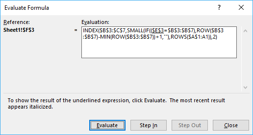
Yous can easily follow forth every bit I explicate the formula, select prison cell D10. Go to tab "Formulas" on the ribbon and press with left mouse push on "Evaluate Formula" push button. Press with left mouse button on "Evaluate" button shown above to movement to adjacent step.

Footstep ane - Identify cells equal to the condition in cell B10

= (equal sign) is a comparison operator and checks if criterion (E3) is equal to values in array ($B$3:$B$seven). This operator isnot case sensitive.

$B$10=$B$3:$B$seven

becomes

"France"={"Germany";"Italia";"France";"Italian republic";"France"}

and returns

{Faux, FALSE, TRUE, Simulated, TRUE}

The epitome in a higher place shows an array in cell range D3:D7 containing boolean values, those values correspond to the logical expression if cell B10 is equal B3:B7. Jail cell B5 and B7 is equal to cell B10, these render TRUE. The other remaining cells is not equal to cell B10 and return FALSE.

Step 2 - Create array containing corresponding row numbers

The ROW function returns the row number based on a cell reference, nosotros are using a prison cell reference that points to a prison cell range containing multiple rows so the ROW role returns an array of row numbers.

MATCH(ROW($B$3:$B$7), ROW($B$3:$B$vii))

The Lucifer function finds the relative position of a value in a jail cell range or array, however, I am using multiple values so this step returns an array of numbers.

Match(ROW($B$iii:$B$7), ROW($B$3:$B$7))

becomes

Match({3, 4, 5, 6, vii}, {iii, iv, v, 6, seven})

and returns {1,2,3,4,5}

The paradigm above shows the array in cell range D3:D7, the array always begins with 1 and has must take the same number of values in the array equally the tabular array has rows.

Footstep three - Filter row numbers equal to a condition

The IF office has three arguments, the first ane must be a logical expression. If the expression evaluates to Truthful so 1 thing happens (statement ii) and if Faux another thing happens (argument 3).

IF(($B$x=$B$3:$B$seven), MATCH(ROW($B$3:$B$7), ROW($B$three:$B$seven)), "")

becomes

IF(Fake, Simulated, TRUE, FALSE, TRUE}, MATCH(ROW($B$iii:$B$7), ROW($B$3:$B$7)), "")

becomes

IF(False, Faux, True, Fake, TRUE},{one, 2, 3, 4, 5}, "")

and returns {"", "", 3, "", v}

The IF part replaces the numbers that correspond to boolean value Simulated with "" (nothing) and boolean value TRUE with a number, shown in cell range D3:D7.

Footstep 4 - Return the k-th smallest row number

To exist able to return a new value in a cell each I use the SMALL function to filter row numbers from smallest to largest.

The ROWS function keeps track of the numbers based on an expanding jail cell reference. It will aggrandize as the formula is copied to the cells below.

Pocket-sized(IF(($Eastward$3=$B$three:$B$7),ROW($B$3:$B$seven)-MIN(ROW($B$three:$B$vii))+ane,""),ROWS($A$1:A1))

becomes

SMALL({"", "", 3, "", five}, ROWS($A$1:A1))

This office of the formula returns the yard-th smallest number in the array {"", "", 3, "", 5}

To calcualte the k-th smallest value I am using ROWS($A$one:A1) to create the number 1.

When the formula in cell D10 is copied to cell D11, ROWS($A$ane:A1) changes to ROWS($A$ane:A2). ROWS($A$1:A2) returns ii.

In Prison cell D10: =INDEX($C$3:$C$7, SMALL({"", "", iii, "", 5} , ROWS($A$1:A1))

=Alphabetize($C$3:$C$7, Pocket-size({"", "", 3, "", five} , 1))

The smallest number in array {"", "", iii, "", 5} is 3.

In Cell D11: =INDEX($C$iii:$C$seven, SMALL({"", "", 3, "", 5} , ROWS($A$1:A2)))

=Index($C$3:$C$vii, Minor({"", "", 3, "", 5} , 2))

The second smallest number in array {"", "", 3, "", v} is 5.

Pace iv - Return value based on row number

The INDEX function returns a value based on a cell reference and column/row numbers.

In Cell D10:

=Index($C$3:$C$vii,three)

becomes

=Alphabetize({"Pear", "Orange", "Apple", "Banana", "Lemon"}, 3)

and returns "Apple" in cell D10.

In Jail cell D11:

=Index($C$3:$C$7,five) returns "Lemon"

This article demonstrates how to filter an Excel defined table programmatically based on a condition using event code and a macro.

Back to top

1.1 Render multiple values - case sensitive

The image above demonstrates a formula in prison cell C10 that extracts values from cell range C3:C7 if the respective value in prison cell range B3:B7 is equal to the value in cell B10.

The values in cell B3:B7  must accept the same upper and lower letters equally the lookup value in cell B10 to generate a match.

Lookup value "france" is found in cell B3 and B7 but not in cell B5. Prison cell B5 has a value that begins with an upper alphabetic character. The corresponding cells to B3 and B7 are C3 and C7, those values are returned in cell C10 and cells below.

Array formula in cell C10:

=INDEX($C$3:$C$7, Pocket-size(IF(Verbal($B$10, $B$iii:$B$7), Match(ROW($B$3:$B$7), ROW($B$3:$B$7)), ""), ROWS($A$1:A1)))

How to enter an array formula

Copy cell C10 and paste to cells below.

If yous own Excel 365 yous tin utilise the much easier FILTER office to attain the same thing: Filter values based on a condition - case sensitive

Back to top

1.2 Return multiple values - if not equal to

The picture above shows an array formula in cell C10 that extracts values from cell range C3:C7 if the respective value in jail cell range B3:B7 is Non equal to the lookup value in cell B10.

The lookup value in cell B10 is non equal to the value in B3, B4, and B6. The corresponding values in C3, C4, and C6 are returned to cell C10 and cells below.

Array formula in jail cell C10:

=Alphabetize($C$iii:$C$7, SMALL(IF($B$10<>$B$3:$B$7, MATCH(ROW($B$three:$B$7), ROW($B$3:$B$7)), ""), ROWS($A$1:A1)))

How to enter an assortment formula

Re-create cell C10 and paste to cells below.

If yous own Excel 365 you tin employ the much easier FILTER function to accomplish the same thing: Filter values if not equal to

Back to top

1.three Return multiple values - if smaller than

The image above demonstrates a formula in jail cell C10 that extracts items from cell range B3:B7 if the corresponding value in cell range C3:C7 is smaller than the value in cell B10.

In the example higher up, cells C5 and C7 are smaller than the value in prison cell B10. The respective cells are B5 and B7 which the formula returns in prison cell C10 and cells below.

Array formula in jail cell C10:

=INDEX($B$3:$B$7, SMALL(IF($B$x>$C$iii:$C$vii, Friction match(ROW($B$3:$B$7), ROW($B$three:$B$7)), ""), ROWS($A$one:A1)))

How to enter an assortment formula

Copy cell C10 and paste to cells below.

If you own Excel 365 y'all can use the much easier FILTER office to accomplish the same matter: Filter values if smaller than

Dorsum to height

1.iv Return multiple values - if larger than

The picture above demonstrates a formula in jail cell C10 that extracts values from prison cell range B3:B7 if the corresponding values in C3:C7 are less than the value in jail cell B10.

In this example, cells C5 and C7 are smaller than the value in cell B10. The formula in jail cell C10 returns the corresponding values from B5 and B7.

Array formula in cell C10:

=INDEX($B$iii:$B$7, Pocket-size(IF($B$x<$C$three:$C$7, Lucifer(ROW($B$iii:$B$7), ROW($B$3:$B$7)), ""), ROWS($A$1:A1)))

How to enter an array formula

Copy cell C10 and paste to cells beneath.

If you own Excel 365 you can use the much easier FILTER function to achieve the same thing: Filter values if smaller than

Back to top

ane.5 Return multiple values - if contains

The image in a higher place demonstrates a formula in jail cell C10 that extracts values from cell range C3:C7 if the respective values in jail cell range B3:B7 comprise the value in cell B10.

In this example, the values in cells B3, B5, and B7 contain the value in jail cell B10. The array formula returns the respective values from cells C3, C5, and C7 to prison cell C10 and cells below every bit far as necessary.

Array formula in cell C10:

=Alphabetize($C$iii:$C$7, SMALL(IF(ISNUMBER(SEARCH($B$ten, $B$3:$B$7)), MATCH(ROW($B$3:$B$7), ROW($B$3:$B$7)), ""), ROWS($A$1:A1)))

How to enter an array formula

Copy jail cell C10 and paste to cells below.

If you own Excel 365 you can employ the much easier FILTER part to achieve the same thing: Filter values if contains

Back to tiptop

1.6 Return multiple values - if non contains

The flick in a higher place demonstrates a formula in cell C10 that extracts values from prison cell range C3:C7 if the corresponding values in cell range B3:B7 do not contain the value in cell B10.

In this instance, the values in cells B4, and B6 do not incorporate the value in cell B10. The array formula returns the corresponding values from cells C4, and C6 to prison cell C10 and cells beneath equally far equally necessary.

Array formula in cell C10:

=INDEX($C$3:$C$7, Small(IF(ISNUMBER(SEARCH($B$x, $B$3:$B$vii)), "", MATCH(ROW($B$3:$B$7), ROW($B$3:$B$7))), ROWS($A$1:A1)))

How to enter an array formula

Copy prison cell C10 and paste to cells below.

If yous own Excel 365 you tin can use the much easier FILTER function to achieve the same thing: Filter values if contains

Back to top

1.vii Render multiple values - that begins with

The formula in cell C10 extracts values from prison cell range C3:C7 if the corresponding values in B3:B7 begin with the same value as the value entered in cell B10.

The paradigm higher up shows that jail cell B4 and B6 begins with the same value every bit the value in cell B10. The corresponding values in cell C4 and C6 are displayed in cell C10 and C11.

Array formula in prison cell C10:

=Alphabetize($C$3:$C$7, Small-scale(IF($B$10=LEFT($B$three:$B$7, LEN($B$ten)), MATCH(ROW($B$iii:$B$7), ROW($B$three:$B$vii)), ""), ROWS($A$1:A1)))

How to enter an array formula

Copy prison cell C10 and paste to cells below as far equally needed.

If you own Excel 365 you lot can use the much easier FILTER part to accomplish the aforementioned thing: Filter values that begin with

Dorsum to height

1.eight Return multiple values - that ends with

Array formula in cell C10:

=INDEX($C$iii:$C$7, SMALL(IF(RIGHT($B$iii:$B$7, LEN($B$10))=$B$10, MATCH(ROW($B$3:$B$7), ROW($B$3:$B$7)), ""), ROWS($A$1:A1)))

How to enter an assortment formula

Copy cell C10 and paste to cells below as far as needed.

If you lot own Excel 365 you can use the much easier FILTER role to reach the same thing: Filter values that cease with

Back to top

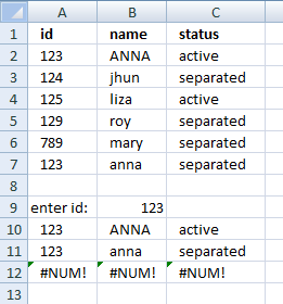
How to remove #num errors

The picture in a higher place shows you the array formula copied down to prison cell D12 however there are simply ii values shown, the remaining cells bear witness nothing not even an fault.

Array formula in jail cell D10:

=IFERROR(Index($C$3:$C$vii, SMALL(IF(($B$10=$B$3:$B$vii), Friction match(ROW($B$3:$B$7), ROW($B$3:$B$7)), ""),ROWS($A$1:A1))), "")

The IFERROR function lets yous convert error values to blank cells or really in whatever value you desire. In this example it returns bare cells.

Note: The IFERROR catches all kinds of formula errors. yous won't spot the error that hands if in that location is some kind of other error in the formula. Use this role with caution.

How to enter an array formula

Recommended articles

How to utilise the IFERROR part  | How to use the ISERROR function | How to use the Error.TYPE function | How to discover errors in a worksheet | Delete blanks and errors in a list

Dorsum to elevation

Count matching values

The following paradigm shows you lot a data set in column B and C. The lookup value in jail cell E3 is used for identifying matching cell values in cavalcade B.

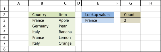
Formula in cell G3:

=COUNTIF($B$3:$B$seven,E3)

Alternative formula in cell G3:

=SUMPRODUCT(($B$3:$B$vii=E3)*1)

Recommended articles

Count a given blueprint in a cell value | Count cells containing text from list | Count cells between specified values | Count entries based on date and time | Count unique distinct values | Count unique distinct records |

Back to top

2 Return multiple values horizontally

Update 17 December 2020, use the FILTER function to return multiple values horizontally. Regular formula in cell C10:

=TRANSPOSE(FILTER(C3:C7, B10=B3:B7))

The formula higher up works only in Excel 365. The assortment formula beneath is for earlier Excel versions and is entered in cell C10.

Array formula in C10:

=INDEX($C$3:$C$7, SMALL(IF($B$10=$B$3:$B$7, ROW($B$3:$B$7)-MIN(ROW($B$3:$B$seven))+1, ""), COLUMNS($A$1:A1)))

Copy cell C10 and paste to cells to the correct of cell C10 as far as needed.

Enter the formula above  as an array formula or utilize this regular simply more complicated formula:

=Alphabetize($C$3:$C$7, SMALL(INDEX(($B$10=$B$three:$B$seven)*(Match(ROW($B$3:$B$7), ROW($B$3:$B$7))+($B$19<>$B$3:$B$7)*1048577, 0, 0), COLUMNS($A$ane:A1)))

Back to acme

Recommended articles

Search values distributed horizontally and return respective values | Resize a range of values | Rearrange values | Rearrange cells in a cell range to vertically distributed values | Rearrange values based on category(VBA) | Normalize information (VBA) | Normalize data, office two |

Extract multiple records based on a condition

Update 17 December 2020, use the new FILTER function to extract values based on a status, formula in cell A10:

=FILTER(A2:C7, B9=A2:A7)

The FILTER part is available for Excel 365 users and the formula above is entered every bit a regular formula.

The formula below is for earlier Excel versions, it extracts records based on the value in cell B9. Array formula in cell A10:

=Index($A$2:$C$vii, Small-scale(IF($B$9=$A$ii:$A$7, ROW($A$2:$A$seven)-MIN(ROW($A$2:$A$seven))+1, ""), ROW(A1)),COLUMN(A1))

To enter an array formula, type the formula in a cell so press and concur CTRL + SHIFT simultaneously, now press Enter once. Release all keys.

The formula bar now shows the formula with a commencement and ending curly bracket telling you that you lot entered the formula successfully. Don't enter the curly brackets yourself.

Re-create cell A10 and paste to cell range B10:C10. Then copy A10:C10 and paste to prison cell range A11:C12.

Picket a video where I explain how to use the array formula and how it works

Enter the formula above as an array formula or use this regular but more complicated formula:

=Alphabetize($A$2:$C$7, SMALL(Index(($B$ix=$A$two:$A$7)*(MATCH(ROW($A$2:$A$7), ROW($A$2:$A$vii)))+($B$9<>$A$2:$A$7)*1048577, 0, 0),ROW(A1)),Column(A1))

Recommended reading

• Extract all rows from a range that meet criteria in ane column
• Match two criteria and return multiple records
• Excerpt records where all criteria match
• Search for a text string in a data set up using an array formula
• Filter unique singled-out records

Dorsum to pinnacle

Lookup and return multiple values [AutoFilter]

The AutoFilter is a congenital-in feature in Excel that allows y'all to speedily filter information. The following video shows you how to rapidly filter a information set, I don't think you tin can practice it more quickly than this.

Instructions on how to filter a data fix [AutoFilter]

1. Press with right mouse push on on a jail cell value that you lot want to filter
2. Printing with mouse on "Filter" and and so "Filter by Selected Cell's Value"
   
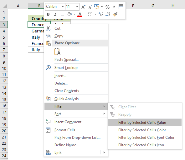
3. That's it!

How to remove a filter

1. Press with mouse on filter button next to header, shown in motion picture below
   
2. Press with mouse on "Articulate Filter From "Country""
   
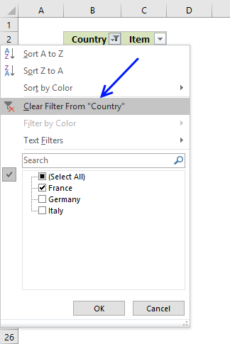
3. The AutoFilter buttons side by side to each header are nevertheless there.
   
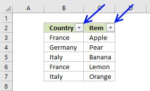
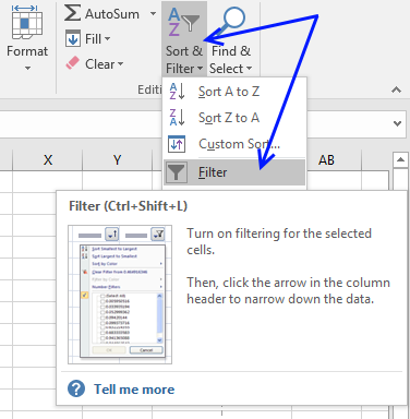
4. If you want to remove those equally well, go to tab "Habitation" on the ribbon and printing with left mouse push on "Sort & Filter" button, then on "Filter"
   
5. The data set now looks like this:
   

Back to elevation

Lookup and render multiple values [Avant-garde Filter]

The Advanced Filter is a tool in Excel that allows you to filter a dataset using complicated criteria combinations like AND - OR logic that the regular AutoFilter tool tin can't accomplish.

In this case I am only going to filter based on a unmarried condition so this will be an easy introduction to the Advanced Filter in Excel.

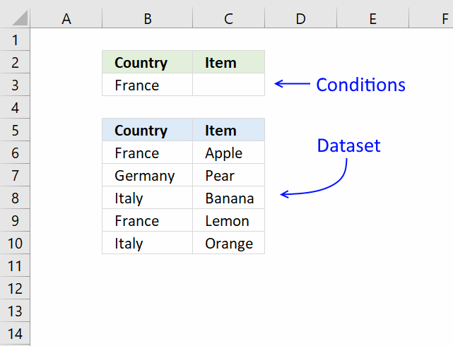
1. Copy the dataset headers and identify them to a higher place or beneath your dataset, this to avoid confusion if the weather condition disappear when a filter is applied.
   Rows will be subconscious and if a condition is on the same row it will exist hidden as well. I created headers on row 2, run into image to a higher place.
2. Enter the condition below the correct header you want to utilise a filter to, I entered my condition in cell B3.
3. Select cell range B5:C10.
4. Go to tab "Data" on the ribbon.
5. Press with left mouse button on "Advanced" push button.
6. Press with left mouse button on in Criteria range: field and select jail cell range B2:C3
   
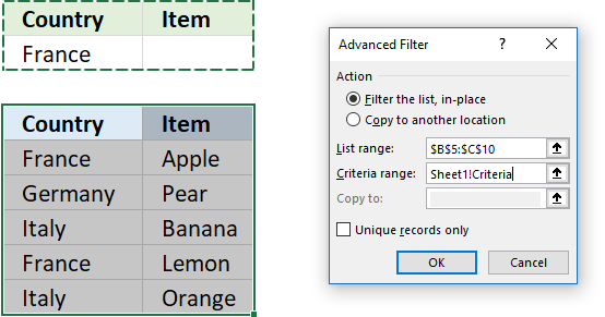
7. Press with left mouse push button on OK button.

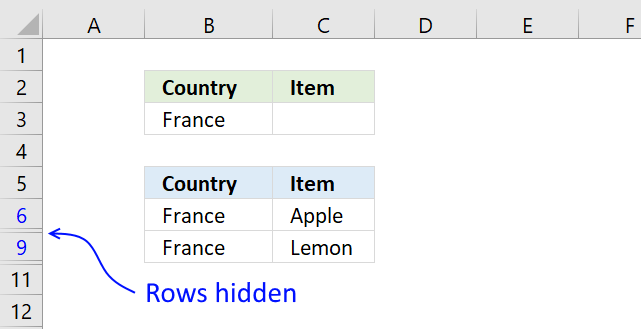
The prototype above shows the dataset filtered based on the condition used in prison cell B3. To clear the filter simply go to tab "Data" on the ribbon and press with left mouse push on "Clear" push button.

Back to top

Lookup and return multiple values [Excel Defined Table]

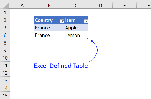
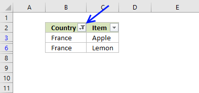
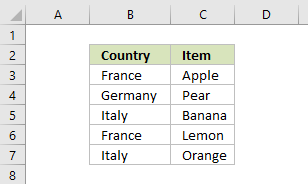
The prototype above shows yous a dataset converted to an Excel Divers Table and filtered based on item "France" in column B.

1. Select a jail cell in your data fix.
2. Printing CTRL + T (shortcut for creating an Excel Defined Table).
3. A dialog box appears, printing with left mouse button on the checkbox if your data set contains headers.
   
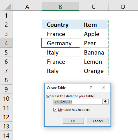
4. Press with left mouse push on OK push.

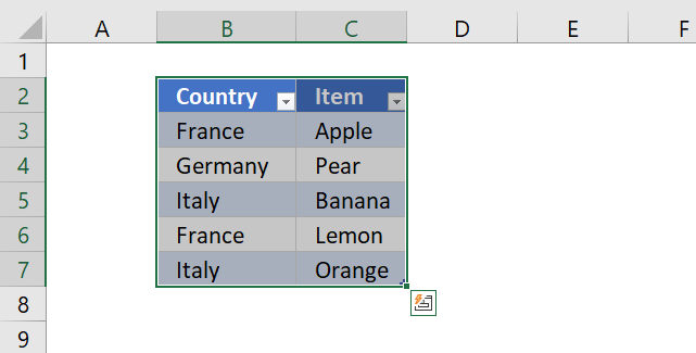
To filter the table follow these simple steps:

1. Press with left mouse button on the black arrow next to a header proper noun.
   
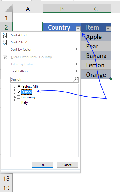
2. Make sure the checkbox next to the value you lot want to use as a status is selected.
3. Printing with left mouse button on OK button.

So why utilise an Excel divers Table? An Excel defined Table contains many more useful features.

• Enter a formula in 1 cell and Excel automatically enters the formula in the remaining Excel Tabular array cells on the same column.
• Jail cell references are converted to structured references, for example a jail cell reference to cavalcade "Country" might look like this: Table[Country].
  This is beneficial because you don't demand to arrange cell references if your table grows or shrinks, the jail cell reference is the same no matter what. You don't need to use dynamic named ranges either.
• Easy to filter and sort data.
• Easy to add or delete data, simply blazon your information beneath the last tabular array row and the Excel defined Table will automatically aggrandize.
• Use as data source for a nautical chart and the chart will brandish what is filtered.

Dorsum to acme

Return multiple values vertically or horizontally [UDF]

Make certain yous have copied the vba code below into a standard module before entering the array formula.

User defined Function Syntax

vbaVlookup( lookup_value, table_array, col_index_num, [h])

Arguments

lookup_value	Required.
table_array	Required. A cell reference to the data table you lot want to search.
col_index_num	Required. A number representing the column in the table_array.
[h]	Optional. Return values horizontally.

Array formula in cell C14:D14:

=vbaVlookup(B14, $B$2:$C$six, 2, "h")

Watch a video that explains how to use the User Defined Function

How to enter custom function array formula

1. Select cell range C9:C11
2. Blazon in a higher place custom function
3. Press and hold Ctrl + Shift
4. Printing Enter one time
5. Release all keys

A beginners guide to Excel array formulas

Dorsum to top

How to enter custom function array formula

1. Select prison cell range C14:D14
2. Type above custom function
3. Press and hold Ctrl + Shift
4. Printing Enter one time
5. Release all keys

How to copy assortment formula to the adjacent row

1. Select cell range C14:D14
2. Copy cell range
3. Select cell range C15:D15
4. Paste

Vba code

1. Copy vba lawmaking beneath.
2. Printing Alt + F11 to open the visual basic editor.
3. Press with right mouse push button on on your workbook in the project explorer.
4. Press with mouse on "Insert".
5. Press with mouse on "Module".
   
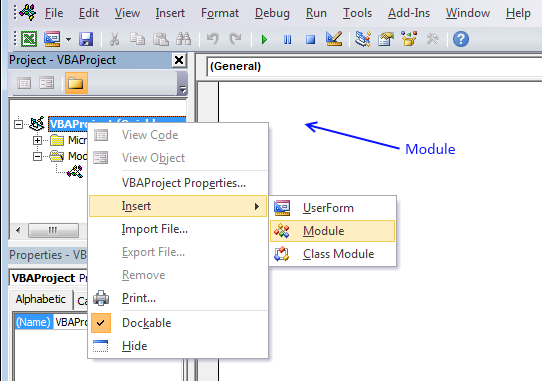
6. Paste code to code module.
7. Get out vb editor and return to Microsoft Excel

'Name User Defined Function and arguments Function vbaVlookup(lookup_value As Range, tbl As Range, col_index_num As Integer, Optional layout As String = "v")  'Declare variables and data types Dim r Equally Single, Lrow, Lcol Equally Unmarried, temp() Every bit Variant  'Redimension array variable temp ReDim temp(0)  'Iterate through cells in jail cell range For r = i To tbl.Rows.Count     'Bank check if lookup_value is equal to prison cell value    If lookup_value = tbl.Cells(r, 1) And so        'Save cell value to array variable temp       temp(UBound(temp)) = tbl.Cells(r, col_index_num)        'Add anoher container to assortment variable temp       ReDim Preserve temp(UBound(temp) + 1)    End If Next r  'Check if variable layout equals h If layout = "h" And so     'Save the number of columns the user has entered this User Divers Role in.     Lcol = Range(Awarding.Caller.Address).Columns.Count        'Iterate through each container in assortment variable temp that won't be populated    For r = UBound(temp) To Lcol               'Salve a blank to array container        temp(UBound(temp)) = ""         'Increment the size of array variable temp with 1        ReDim Preserve temp(UBound(temp) + ane)    Next r     'Decrease the size of array variable temp with one    ReDim Preserve temp(UBound(temp) - 1)     'Return values to worksheet    vbaVlookup = temp  'These lines will be rund if variable layout is non equal to h Else     'Save the number of rows the user has entered this User Divers Function in    Lrow = Range(Application.Caller.Address).Rows.Count     'Iterate through empty cells and save zilch to them in gild to avoid an error being displayed    For r = UBound(temp) To Lrow       temp(UBound(temp)) = ""       ReDim Preserve temp(UBound(temp) + one)    Adjacent r  'Decrease the size of assortment variable temp with 1 ReDim Preserve temp(UBound(temp) - 1)  'Return temp variable to worksheet with values rearranged vertically vbaVlookup = Application.Transpose(temp) End If  End Office

Recommended reading

• Lookup multiple values in one cell [UDF]
• Fuzzy lookups [UDF]
• Filter an Excel defined Table based on selected prison cell [VBA]
• Filter words containing a given string in a prison cell range [UDF]
• Filter an Excel defined Tabular array programmatically [VBA]
• How to save custom functions and macros to an Add-In
• Add your personal Excel Macros to the ribbon

Dorsum to height

Back to top

hallwhouse.blogspot.com

Source: https://www.get-digital-help.com/how-to-return-multiple-values-using-vlookup-in-excel/

Share this post